Histogram Manipulation

It's pretty hard to take pictures at night, images will most likely be dark. I think many will agree with me.. the fun starts at night (just to be clear.. I'm not a party person but I do believe that people had their most fun happenings at night)! But what if your only-once-in-a-lifetime captured moment turnout dark? Worry not! :) Scilab, or for the simplest way possible, advanced image processing software like GIMP has a solution for that :)

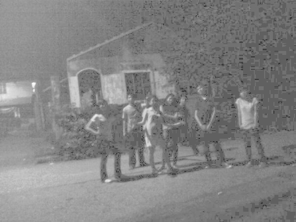
Every images, when in grayscale, has its histogram. It is the Probability Distribution Function (PDF) of the image that lets you identify the tonal distribution of an image. Even those dark-looking images still contain information, they were just in the darker range. If the PDF is modified, enhancement on the image can be done.. dark images could look brighter, etc. For our sixth activity, we are asked to enhance pictures through histogram manipulation. This was done by "backprojecting" the grayscale values into the desired Cummulative Distribution Function (CDF) using the CDF of the PDF of the original image.[1,2] This will be further discussed later on. Let us consider this picture. 

Using Scilab, the image was converted to grayscale using the function rgb2gray() and the resulting image is seen below. 

Then, histogram of the grayscaled image was obtained using imhist() function. Scilab Help would always make our life easier. The variable hist that I used in the code (seen far below) represent the distribution itself and the cells are the bins. Unless specified, the bins of the histogram were set in default, which is 256 given the type of our image. So we can plot hist vs. cells or just plot(hist). But to produce a normalized plot, the histogram must be divided by the total number of pixels of the image. The normalized histogram is shown in the figure below

CDF of the histogram was obtained using the function cumsum(). Again normalizing, CDF resulted to the following plot

As you can see, the pixels were concentrated on small values. We want the values to be equally distributed implying that there would be the same amount of dark and light colors. For the desired equally distributed histogram, the CDF is linear as shown in the figure below. Human eye, on the other hand, does not have a linear response. So we will try other CDF - one that represents a sigmoid function. Backprojecting was done by finding the corresponding y-values of the original CDF to the desired CDF then replacing the pixels value with the x-values from the desired CDF. [1]

The desired CDFs showing a linear function (left) and sigmoid function (right). 

I understand well the concept of backprojecting. However, I really have a problem on incorporating it into a code. Ma'am Soriano suggested to use interp() function but it's really hard for me to figure out the correct syntax. For that, I'm really thankful to Nestor Bareza (for like always willingly helping me :)) I also thank Joshua Beringuela for the helpful discussion about the find() function. 

Now the enhanced images are as follows:

Enhanced image using a linear CDF. 

Enhanced image using a sigmoid CDF. 

Comparing with the grayscale of the original picture, the brightening up of the photo was evident. It was observed that for the enchanced image using linear CDF was lighter and revealed more details than that of the sigmoid CDF. Also, to check, the PDF and CDF of the enhanced images are shown below. The CDF of the enhanced image somewhat follows its desired CDF.

PDF of the enhanced images using a linear CDF (left) and sigmoid CDF (right). 

CDF of the enhanced images using a linear CDF (left) and sigmoid CDF (right).

The complete code:

Now using GIMP to modify the histogram..

So I guess the class' favorite subject in this activity is our very handsome classmate, Nestor :P So I thought of doing the same :)

Histogram manipulation can also be done using GIMP. From colors menu, just click the curves. This is the original image with the linear curve..

Adjusting the  curve...

Oops! wrong move. undo undo. Our lovely Tor would not be pleased. hehe

Okay, better :) So yah! You can't really resist this beauty and hotness. XD

If the concavity of the curve shifts upward, the image becomes darker. What you want is the downward concavity in order to make the picture appears brighter and reveal more details. Trying a different curve, image will look something like..

It can also be performed using other freeware image processing software.. so I have Paint.NET installed in my laptop, better try it out! :) The picture of the Siene River with Eiffel Tower in the view is obtained from [3]. Exploring the menus and tools, you would find in Adjustment menu the Curves and just like in the GIMP it can be adjusted.

So yes, it worked just like the GIMP. And again playing with the curve..

Tadah! A pretty nice color combination :)

I'm giving myself 11/10 for successfully enhancing the pictures through their histogram and employing this on other freeware software, Paint.NET :)
__________
References

[1] Soriano, M. "Enhancement by Histogram Manipulation." AP 186 Laboratory Manual. National Institute of Physics, University of the Philippines, Diliman. 2013.

[2] Image Histogram. Retrieved from http://en.wikipedia.org/wiki/Image_histogram
[3] http://shedexpedition.com/wp-content/uploads/2013/05/France-Eiffel-Tower-and-the-Seine-River-at-Night.jpg