Neural Network

Using the features from the pattern recognition activity, classification can be done using neural network. For this activity, the result is still not what is expected and still need to improve the training

For now... here are my results for the training set

Even when binary numbers were used, still the result was not what is desired for the training set.

__________

References

[1] Soriano, M. "A15 – Neural Networks." AP 186 Laboratory Manual. National Institute of Physics, University of the Philippines, Diliman. 2013.

Pattern Recognition

Human can easily identify objects and we've been able to do this by looking for object features or patterns like color, shape, size, etc. The process of identifying objects through the use of computer is of major interest in Pattern Recognition. To be able to imitate this complex ability of humans would be amazing. In the next generations, we will have our computers do everything for us.

In pattern recognition, two steps are involved - feature extraction and classification. Choosing the feature of the object is crucial for distinguishing it from the set of classes. I choose the set of cereals with the three classes: honey gold flakes, koko krunch and honey stars. The feature that obviously differentiate the three classes is the color. Actually, it's been hard for me to choose my classes. It's either not good for classification or been taken already by my classmates.

Figure below presents the training set.

Figure below shows the plot of features of the cereals based on color (red and green chromaticity value). The X marks represent the mean points of each class. 

Now for the test set, the comparison of the distance measurement will be able to classify the cereal. The one having shortest distance from the test object will be the predicted class. Table below shows the predictions. 

Out of 9 test objects, 7 were correctly predicted, that is 77.8 % accuracy. Color feature were fairly enough to differentiate the cereals however, I think the prediction would be more accurate if more features were extracted like the eccentricity since the stars would have big difference on the eccentricity of the circle cereals. However, I lack the time to do another feature extraction so I sincerely apologize for disappointing my readers. :P 

I give myself a grade of 9/10 for at least doing the objective of the activity even I only extract one feature which is the color. 

__________

References

[1] Marcos, S. and Soriano, M. "A14 – Pattern Recognition 1." AP 186 Laboratory Manual. National Institute of Physics, University of the Philippines, Diliman. 2013.

the following sites are where the cereals pictures are taken
http://breakfastlullaby.blogspot.com/2012/11/nestle-honey-gold-flakes.html

http://www.seriouseats.com/2012/07/3-cereals-from-singapore.html
http://fun-fanie.blogspot.com/2011/01/di-saat-kehamilan-begini-makanan-yang.html
http://wayfaringchocolate.com/2012/03/29/march-bits-and-bobs-pancakes-asian-sweets-and-advice-we-
http://nicolekissdiet.blogspot.com/2008/02/koko-krunch-duo.html

Not Just Your Usual Image Compression

In this activity, an image is compressed in not just the ordinary way that you know. The main reason why we want to compress images is to reduce the image size. Our cameras are continuously advancing and the information that it can gather from the object are almost limitless, in other words, high-def. But some information are not necessary. On way of compressing image is through principal component analysis (PCA). [1]

To clearly demonstrate the compression, I use a very large image of a clownfish taken from National Geographic website [2] as shown below. It has a dimension of 1600 x 1200 pixels and size of 2.12 MB - truly a BIG image. However, the very big original image encountered a problem on the working stack size in the Scilab. Even I maxed out the stack size, it really wasn't able to operate on very large scale. So, I need to resize the image to 800 x 600 pixels resulting to size of 388 KB - still relatively large.

The image was first converted to grayscale. The image was then cut into 10 x 10 pixels subblocks then concatenated into single column matrix with 100 elements. The concatenated subblocks was arranged into n x p matrix x where n is the number of subblocks and p is the number of elements in each block. We then get the pca of x. In Scilab, the following line was used.

[lambda,facpr,comprinc] = pca(double(x))

The facpr matrix contains the eigenvectors or eigenimages that composed the image, with the first column to have the highest contribution or weight to the original image and so on. The eigenvalue or the constant value

From the grayscaled image below...

the reconstructed images using different numbers of eigenimages are presented. From the lamda, the corresponding weight of each eigenimages was known. The cumsum() function will determine how many eigenvectors will achieve a specific percentage in reconstruction. One eigenimage already correspond to 95.1% of the original image. On the other hand, using 5, 20, 85 and 100 eigenimages result to 97.9%, 99.0%, 99.9% and 100% of reconstruction, respectively. 

For each reconstruction, compression of the image were made. From the grayscaled image original size of 183 KB, the reconstructed images resulted to decrease in size to 89.0 KB, 80.8 KB, 94.5 KB and 174 KB using 1, 5, 20 and 85 eigenimages, respectively. The decrease were 51.4%, 55.8%, 48.4% and 4.9%.

Using all 100 eigenimages (100% reconstruction), doesn't have much difference from when 85 eigenimages were used. Also, no compression had took place. The image size resulted to 183 KB, the same size as the original image. 

Now, let's put some colors to our reconstruction

The image size resulted to 112 KB, 97.6 KB, 114 KB and 195 KB. From the original 388 KB image size, the percent decrease were 71.1%, 74.8%, 70.6% and 49.7%. The compression was observed to be greater for the colored image. 

I thank Phoebe for helping me debug my code. I am giving myself a grade of 11/10 for accomplishing the goal of the activity and doing the reconstruction in colors. 

__________

References

[1] Soriano, M. "A13 – Image Compression." AP 186 Laboratory Manual. National Institute of Physics, University of the Philippines, Diliman. 2013.

[2] Clownfish and Bubble-Tipped Anemone. Photograph by David Doubilet. Retrieved from 
http://photography.nationalgeographic.com/photography/photo-of-the-day/clownfish-bubble-tipped-anemone/

The code of music

Going over the title, you may misunderstand the point of this blog post. So I will have to tell it as early as now. This is to producing music through Scilab. Yes! Some functions will be able Scilab to sing. I will just be simple but what we want to accomplish in this activity is to make the Scilab read the notes in a music sheet.

I am a frustrated pianist. I was taught to play piano when I was in elementary but things (like my laziness and impatience in learning.. well I'm just a kid then so I do have more significant matters to be taken care of :P) lead to another path and I wasn't able to learn much. Well, I regret missing that chance because I really have a passion for music. It just that I am not the best suited for it so let's just stay admiring these work of art. :)

At first, I really thought that it would be tedious in making this activity work. I listed below some of the things that I think what are needed to be considered.

(a) make the Scilab know the pitch of the note (if a C, D, E, etc);

(b) make the Scilab know the tempo of the note (or the duration, depends if a whole note, quarter note, etc.); which will both require to

(c) have the right filtered image

Better start losing sweat! The song that I chose is Old MacDonald, one simple nursery song because we don't want to make our life more difficult. Below is the music sheet for Old MacDonald in C Major [2]. Again this is simple because there were no flats and sharps :)

The music sheet was first cropped so we can handle on the first line for the mean time.
 

The image must be binarized first, if it is not a binary image. Then the color of the image was inverted. As I worked through my code, the task seems more problematic than I thought. The first problem that I encountered: problem (c) or filtering the image. I instantly thought that using a circle structuring element then applying open operator would isolate the notes. It pretty much did however, the half note would not be included. So I think of another way. It was to remove the vertical and horizontal line. Shown in below is the step by step cleaning of the image. First, removing the vertical, then horizontal lines, both using the TopHat() function. Unfortunately, there really parts of the note that would be removed in performing these steps so the CloseImage() function was used.

I will now be having my blobs and using the FilterBySize() would remove the unnecessary small blobs. We now have the following blobs.

We now arrive to problem (a) mentioned above. How will the Scilab know the ptich of the note? In the music sheet, the pitch was differentiated through the location of the note in the staff (the one with the five horizontal lines). Thus, those position should also be recognized by the Scilab. AnalyzeBlobs function in Scilab measures the location of the centroid of each blob. In Gimp, the range of pixel location of each line and space along the y-axis were determined. These were incorporated as conditions for the Scilab to know the right pitch. We should now face problem (b). Since, half notes are not solid circles, we can deduce that their areas are different from the quarter notes. So again, conditions were made to determine the tempo.

The whole process of making the Scilab read notes seems successful. Below is the output.

This task really has been tedious. I spend a lot of time in determining the location range because the you have to consider that there are different range for spaces and lines. Though once established correctly, you're okay. For the next line, however the next staff will be another problem because the pixel position or ranges of spaces and line would be different when another cropping of image was made. The practical thing to do is to work to match the pixel positions of spaces and lines of each staff. In addition, working on the tempo is really a killer. I am lucky that the first staff only contains only half and quarter notes. I able to distinguish between the two notes. There still whole, eighth and sixteenth notes and the dot beside the note. The eighth and sixteenth notes is notable for the one bar and two bars above their musical symbol, respectively. I plan on working on those by determining their position along the x-axis and if they are reasonably close to the blob representing the note, the tempo of the note will be known. Still, these need a lot of work to be accomplished. Maybe I'll try it when I had the time, including the rests in the music scores.

I am thankful for the initial code that Ma'am has provided us that make the Scilab produce different pitch. I also thank Aeriel Constantino and Phoebe Gallanosa for the useful discussion. I believe I deserve a 10/10 in this Activity because technically, I accomplished the task at hand.

__________

References

[1] Soriano, M. "Playing Notes by Image Processing." AP 186 Laboratory Manual. National Institute of Physics, University of the Philippines, Diliman. 2013.
[2] http://www.pianolessons4children.com/songs/old-mcdonald.php
[3] http://www.ukuleles.com/spreadsheets/Guitnote.XLS (for the frequency of other pitch)

Blob Analysis

Sometimes, we would like to get measurements from images and the process would be easier if the region of interest (ROI) is clearly distinguishable from the rest of the image. In other words, we want our ROI to be well-segmented from its background and it can be achieved by edge detection or by specifying the ROI as a blob. Either way, the images must be first undergo preprocessing in order to make them more suitable for performing the desirable measurements. This activity makes use of blobs to analyze the 'cells' found in the image.

Determining the best estimate of area of the cells

In image processing, blob is considered to be a region of connected pixels. In Scilab, blobs are detected from binary images which exclude them to the background pixels or those having zero values. You can see below the image of white circles which we consider the cells

To process the images easier and faster, it was cropped into 256x256 pixels subimages. The image was cropped using GIMP and we allowed overlapping subimages. This resulted to 12 subimages.

One subimage (upper left part of the whole image) is shown below.

Subimage 1.

To segment our regions of interest, we need to binarize the image. We have to consider the histogram of the image in order to determine the enough threshold value to produce an output image that will best isolate our cells and background. I first used the usual imhist() function and obtain its peak for the threshold but it was tiring and time consuming given that we have 12 subimages. So it was grateful to know that Scilab has all its way of making our image processing easier :). As I explored the Image Processing Design (IPD) module of Scilab, I came across the CalculateOtsuThreshold() and SegmentByThreshold() functions. (IPD is available on ATOMS Module Manager of Scilab. You would only need to install it manually.) The first function is able to solve the threshold of the images automatically while the latter is used to binarized the image with the set threshold value

We favor the values higher than the threshold to clearly represent the cells, just don't make it so high that everything would appear black. So in binarizing the image, we add 20 to the calculated threshold value. This resulted to more distinguishable ROI and background. The comparison of using different threshold values can be seen below.

Converting the image to its binary image with threshold equal to the image threshold value (left) and threshold+20 (right).

Seen below are all the binarized subimages

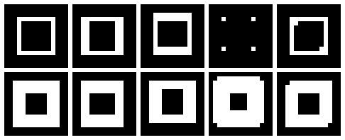
However, this image cannot still be used for measurement analysis because this is still 'dirty'. With the use of morphological operation done in the previous activity, the image can be further cleaned up. Understanding the closing, opening and tophat operator, the image can be cleaned nicely. I really had a hard time doing this part because there were a lot of factors to consider. First, was the structuring element to be used then you would then think of the right combination. I understand well the use of the closing and opening operator because its name was already self-explanatory, while the tophat operator is just confusing. So I decided not to use it in this activity :P

A sample of the cleaned image applying closing operator first (left) then open operator (right).

I realized that the structuring element that I need to use was a circle, the same shape as our cells. The only problem is the size. I first use the CloseImage() function so that our ROI will fully cover our cells then OpenImage() function was used to separate adjacent cells. This separation was only effective for cells nearly touching each other but for overlapping cells, it just doesn't do much. However, this operator was still useful because this make the excess dirt pixels in the background to be wiped out. See image above :)

Shown below are all the cleaned subimages.

Now, we can now analyze our blobs. SearchBlobs(), another function of IPD, was used to assign numbers to each blob found in the image. Now, each blob can be called separately, thus will able to analyze its features like area.To ensure that the blobs have their own individuality, the ShowImage() function was used resulting to the graph of blobs respresented with different color. And just for the heck of trying, I tried the the bounding box feature, which can all be found in the blob analysis in the IPD module.

The area of each blob can be easily computed using the size or the length function however, the area of each cell cannot be obtained because not all the blobs represent only one cell as what is observed on the blobs on the right portion of the images above. So I establish a code that if it consider the the blob contains two cell, the area will be divided by two, and so on. I completely understand that this procedure will make the estimate inaccurate but this was the best solution that I could think of.

Table below shows the area computed for each blob of each subimages.

From all these data the computed mean and standard deviation were 525.69605  and 94.437235, respectively. The calculated best estimate of the area of the 'cells' is

Isolating the cancer cells from the healthy ones

Using the best estimate, the cancer cells, represent by abnormally large size cells, can be isolated from the normal cells. The image containing both cancer and normal cells is shown below.

Doing the same process in first image, we search for the blobs in this second image. I just processed the image as it is, without any cropping. The binarized image and the cleaned image are shown below

I isolated the cancer cell simply by using the FilterBySize() function of the Scilab with bounds of [431, 620] repesenting the range of the best estimate of the area. The result is as follows.

This looks pretty much right. The cancer cells were removed however other normal cells were also removed. The cells that was taken out was displayed by setting the parameters of FilterBySize() greater than the best estimate bounds.

So, yes! There were normal cell that be removed. The same as the problem previously, there were overlapped cells and since they were big, the code consider it as cancer cell.

I give myself a grade of 10/10. I wasn't able to produce the desired output but I give myself a consolation point for exploring other stuff and the product of real hardwork :)

__________

References

[1] Soriano, M. "Application of Binary Operations 1 : Blob Analysis." AP 186 Laboratory Manual. National Institute of Physics, University of the Philippines, Diliman. 2013.

This been an exhaustingly dull weekend and weekdays. The rain just really set the mood a little off. I've been confined inside my room for like countless days, sitting in front of my computer doing my blogs and papers, or listening to music, or watching TV, and just going outside in need for food. And whenever I see bad news concerning the storm, I can't help but feel down.. especially if the news is about your province. Bataan is now under state of calamity and all I can is pray for the safety of my friends and loved ones. Stay safe everyone!

Morphological Operations

Morphology refers to the study of shapes, forms and structures. Classically, morphological operations are done on binarized images. By applying different morphological operations, the images were modified. The were a lot of possible outcome on the image, may be narrowed, widened, hole may be filled or connected blobs may be separated.

Some of the morphological operations were erosion and dilation.

Erosion operator is defined by

The product of the erosion is to reduce the image A by the shape of B. The image should obviously be narrower or thinner.

Dilation operator is defined by

The product of the dilation is to expand the image A by the shape of B. The image should obviously be thicker or wider.

The images to be applied with morphological operations are as follows:

1. A 5×5 square
2. A triangle, base=4 boxes, height=3 boxes
3. A hollow 10×10 square, 2 boxes thick
4. A plus sign, one box thick, 5 boxes along each line

The structuring elements to be used, on the other hand, were the following

1. 2×2 ones
2. 2×1 ones
3. 1×2 ones
4. cross, 3 pixels long, one pixel thick
5. A diagonal line, two boxes long

Erosion and Dilation results

The set of erosion and dilation results includes the one done by hand (graphing paper images) and the other using Scilab functions.

Erosion and dilation of a 5×5 square by the set of structuring elements

Erosion and dilation of a triangle, base=4 boxes, height=3 boxes by the set of structuring elements

Erosion and dilation of a hollow 10×10 square, 2 boxes thick by the set of structuring elements

Erosion and dilation of a plus sign, one box thick, 5 boxes along each line by the set of structuring elements

The predicted result were all matched with the code-simulated result. With this I give myself a grade of 10/10 by accomplishing all the required output.

________________________
[1] Soriano, M. "Morphological Operations." AP 186 Laboratory Manual. National Institute of Physics, University of the Philippines, Diliman. 2013.

Color Picker

In an image, an object or a portion can be segmented from the rest of the image by considering its color. From the image below, the green cap was the one to be segmented. 

The Region of Interest (ROI) that was picked from the image is shown below

Using Scilab, the red, green and blue channel or component of the image is separated. The raw RGB values were transformed to its normalized chromaticity coordinates (NCC) using the equations below

where I = R+G+B is the intensity value of the color.


Parametric Probability Distribution Estimation

Each pixel of the ROI has its rgb chromaticity values. This segmentation makes use of the mean and standard deviation of the rgb chromaticity values of the ROI. The probability of each image pixel with chromaticity r that belongs to the color distribution of the ROI is defined by

similar equation is done for the probability having chromaticity g.The joint probability results to the final segmented image, which for our image is shown below. 

Non-parametric Probability Distribution Estimation

Non-parametric segmentation is done by getting the value of each pixel of the ROI. The values were plotted in the 2D histogram. A certain color has its certain location in the NCC color space. The 2D histogram of our ROI is represented below. The white patch in the histogram was observed to agree with the desired location of the green in the NCC space. 

The 2D histogram was used to backproject the values to the whole image. The value of each pixel of the image were located in the histogram and whatever the values in that location will be the value replaced in that pixel. The result of the non-parametric color segmentation is as follows. 

For both of the color segmentation, however, not the entire cap was segmented. The portion that was not segmented were the darker shades of green. Making the ROI cover a bigger area to better represent the color, especially those of lower brightness, the figure below shows the new ROI and its corresponding 2D histogram. 

The output of the parametric and non-parametric color image segmentation is as follows. It was observed that when the ROI is made bigger, which better represents the all the shades of color of a region, the segmentation is improved. 

Output of parametric (left) and non-parametric (right) color image segmentation

Let's try for other picture :)

I try to isolate each color..

This technique really have amazing results. The upper set is the parametric while the lower set is the non-parametric color image segmentation.

In my outputs, it was observed that non-parametric segmentation better and cleaner segmentation. Also, it is faster since no computations of mean, standard deviation and probabilities were need to do the segmentation. 

I give myself a 11/10 for accomplishing the desired result. Additional points for trying to make the ROI bigger and applying the segmentation is many other objects. 

________________________
[1] Soriano, M. "Color Image Segmentation." AP 186 Laboratory Manual. National Institute of Physics, University of the Philippines, Diliman. 2013.