Neural Network

In this activity, the task is to apply neural network in any classification. In a previous activity, pattern recognition was used to classify three different cereals using r ang g normalized chromaticity (ncc) values as features. You can view that activity here.

Figure below shows some of the samples for our classification. The complete set composed of 24 samples, 8 for each class - honey gold flakes, koko krunch and honey stars. 

To easily classify objects using machine learning, the combination of features to be selected should discriminate well the classes. Using only colors as features will be a weak classification technique. In the previous activity, there's a difficulty in the distinction between corn flakes and honey stars since they have similarity in their color. To strengthen the classification, we can add other features concerning the shape of the cereals. The edge of the samples are obtained using Matlab. Based on the edge or boundary another two features are obtained. 

Roundness is given by[1]

$$Roundness = \frac{4\pi A}{P^2}$$

where A is the area of the edge shape and P is the perimeter of the contour. 

Solidity is defined as the ratio of internal and external area[1]. 

$$Solidity = \frac{S_1}{S_2}$$

where $S_1$ and $S_2$ is the internal and external area of the shape, respectively as illustrated in the figure below[1]. 

From these additional features, we can easily differentiate corn flakes and honey stars. The stars will have low roundness and solidity. 

Now that we have five features to classify our cereals, we use an existing package for neural network in Matlab. Here the network was trained using Levenberg-Marquardt backpropagation. We observe the different result of the fitting using different number of hidden neurons. 

The error histogram using 10 hidden neurons is used. In the histogram, one can observe if there's any outliers[2]. For this case, the error seem close to each other with most errors within -0.06 to 0.04. 

Using 50 and 100 hidden neurons, the resulting error histogram is as follows. 

For these cases, it was more apparent that the data has outliers and this would indicate that there are some of the data are not valid or if they are valid, the guide suggests to collect additional data that are similar to the outlier points[2]. This error histogram will indicate whether our data or selected features is suitable enough for neural network classification. 

The plot above shows the different regression plots. This shows the linear relation between the outputs and the target for the training, validation and test sets[2]. In the neural network, we should observe linearity between network outputs and target. The best linearity was observed using 100 hidden neurons. 

Retraining the data set doesn't really improve the result. Actually, every training seem to be very different from the each other. But the error seem to be relatively smaller using higher hidden neurons. From our data so far, we can say that mostly have low error with some possible outlier data points. 

--

Reference

[1] Q. Wu, C. Zhou, and C. Wang, "Feature extraction and automatic recognition of plant leaf using artificial neural network," Advances in Artificial Intelligence, 3, 2006. 

[2] N.A., "Fit Data with a Neural Network," MathWorks, Inc., 2016. <http://www.mathworks.com/help/nnet/gs/fit-data-with-a-neural-network.html>

Matlab has an existing package for neural network.

Here the network was trained using Levenberg-Marquardt backpropagation

Apply NN in any classification or fitting task. You need not program from scratch, use existing packages. Play around with free parameters such as number or hidden neurons, number of hidden layers, activation functions and learning algorithms.

Face Tracking by Skin Color Segmentation

Face tracking from image frames or videos may be done by finding a way to segment the skin from the image frames. In this activity, the segmentation of the skin was done using non parametric color image segmentation. Parametric and non parametric color image segmentation were already done in the previous activity. You can find it here for more detailed implementation of the color image segmentation.

Initially, we captured a video of ourselves as we move from one lighting condition to the other. It is observed that the color of the skin changes for different lighting conditions. Some frames in the video was chosen to represent each of the lighting condition. In the method, skin patches were cropped under the different lighting condition and the histogram of the skin patch was plotted in rg normalized chromaticity space. I first obtain the histogram of the skin under sunny lighting condition, as shown in the figure below. 

Histogram of skin under sunny lighting condition.  

This histogram was used to segment the skin on the background. Histogram backprojection was used to replace the value of every pixel location of the image frame by the corresponding value of its location on the histogram. After backprojecting, the resulting image was thresholded with just a small value of 0.005 to remove those pixels that have very small possibility of belonging to the skin segment, Using blob analysis, bounding box was placed around the blob that has the largest area. The result of the backprojection on an image frame, the thresholded image, and the image that has a bounding box representing the largest blob area are shown in the figure below. 

The bounding box representing the largest blob will also serve as the detected face during the face tracking (since, of course, our face consists of mostly skin). The histogram of the skin under the sunny lighting condition was used to image frames that are under other lighting conditions. The figure below illustrate the resulting face track and as predicted, the face was not able to recognize on the cloudy and/or dark lighting condition. Also, we note that the face that was tracked under the fluorescent lighting condition seems smaller. 

We now consider the histogram of the skin under different lighting conditions including sunny, cloudy, fluorescent and dark. The histogram is presented below and it was observed that the skin locus now covers a big area on the 2D histogram plot. 

Histogram of skin under differen lighting conditions.

The resulting face tracks were now also to recognize the face under different lighting condition and the bounding boxes were observed to be able to enclose the entire face (or the entire skin patch) on the image frames under different light conditions. 

The final output of the face tracking of the image frames in the whole video is now presented below. 

Final Output

--
Reference
[1] Soriano, Maricor, et al. "Adaptive skin color modeling using the skin locus for selecting training pixels." Pattern Recognition 36.3 (2003): 681-690.

Texture Recognition

One way to analyze the texture pattern in an image is through Local Binary Pattern (LBP). The computation of the LBP is done as follows:

(1) for every pixel location, get the difference of the center pixels from each of its eight neighboring pixel.
(2) set a threshold in which all the negative values are zeroes, otherwise ones.
(3) set a fixed weight for each of the 8 position of the neighbor, that is, $2^{n-1}$ for the nth neighbor where the movement is in clockwise direction.  Multiply this weight to the corresponding thresholded values.
(4) compute the sum of these products. The sum is the LBP value for that neighborhood.

The summary of the computation of LBP is illustrated in the figure below

Three texture classes that were considered for this activity are sand, sponge and wood. At least five samples for each class were considered. The first set of texture samples is shown below. 

Sand texture samples in grayscale. 

Information about the texture are presented here through histogram. The LBP histogram for each sample of the sand texture is shown below. Aside from the peak at the very dark and the very light values or the two ends of the histogram, the other bins don't have drastic difference in values. This histogram pattern was consistent for all five sand samples. 

LBP histogram of five sand texture samples.

Sponge texture samples

Sponge texture samples in grayscale.

The LBP histogram for each sample of the sponge texture. Ideally, different texture have different histogram. The difference of the sand LBP histogram between the sponge LBP histogram are easily noticeable. The histogram of the sponge texture as shown below have sudden drop and rise in their values but this is relatively the same result for all five sponge textures. 

Wood texture samples

Wood texture samples in grayscale.

Lastly, the LBP histogram for each sample of the wood textures was acquired. It was observed from the figure below that the three fork shape at the middle was prominent for all the histograms. But for other part, we can reasonably say that they are similar to each other. 

But for strong argument sake, I presented below their corresponding histograms using smaller bins for this set of texture. Now, we can observed the similarity between the five histograms better. The middle values have relatively negligible density as compared to the rest where the the right side seems to have heavier weight than the left side. This is different from the other textures because the LBP histograms of sand and sponge have pretty much symmetric right and left sides.

References

[1] Matti Pietikäinen. Local Binary Patterns. 2010. http://www.scholarpedia.org/article/Local_Binary_Patterns

Invariant moments

Computing the moments of invariant is a way to recognize the visual patterns and characters independent on its position, size and orientation[1-2].

The moments of invariant of images were computed in this activity. We have a set of images which consists of the original image, rotated image and scaled image. Consider first a set of grayscale images as shown below.

Set of grayscale images. Original image, rotated image, and scaled image (from left to right) . 

The 2D moment of order (p+q) of an image was given by
$$m_{pq} = \sum_{x=0}^{N-1} \sum_{y=0}^{M-1} x^p y^q f(x,y)$$
The central moment is then given by
$$\mu_{pq} = \sum_{x=0}^{N-1} \sum_{y=0}^{M-1} (x-\bar{x})^p (y-\bar{y})^q f(x,y)$$
where $\bar{x}$ and $\bar{y}$ are calculated using the following equations
$$\bar{x} = \frac{m_{10}}{m_{00}}; \bar{y} = \frac{m_{01}}{m_{00}}$$
The normalized central moments $\eta_{pq}$ is now computed as
$$\eta_{pq} = \frac{\mu_{pq}}{\mu_{00}^\gamma}; \gamma = \frac{p+q}{2} +1$$

From the second and third order of moments, a set of seven invariant moments was derived.

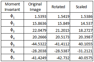
In matlab, the computation is done using for loop to access each pixel position and the value of the image in that position. The calculated invariant moments for the grayscale image set are summarized in the table below. For each invariant moment, the values are nearly the same for the three images. The closely similar values of the invariant moments just justifies that the images are recognized to have the same pattern regardless of the rotation and the size.

The same procedure was done for other set of images. Unlike the grayscale images which have an image function $f$ that ranges from 0 to 255, the succeeding sets of images are binary images which have values that are only either 0 or 1. Edge images are like Dirac delta function which has peak values (equal to 1) located at the edge otherwise, the values were zero. 

I applied the same procedure first for my chromosome edge image in the last activity but the resulting invariant moment values were not that similar to each other. When discussing with Anjali, she thought that maybe there were too little details that this approach wasn't able to recognize the patterns. So I tried other edge image that have a many details as shown in the figure below. 

The values of the moments invariant for the set of edge image are tabulated below. Now, the values for each moment invariant were observed to be closely similar. And since the edge images are mostly zeros in values, the invariant moment values are also smaller as compared to that of the grayscale set of images. The eight invariant moments for this set is just in the range of [0.2, 7.4].

Lastly, the moments invariants for the set of synthetic symmetric images were also computed. They were like step function which have zero values for the background, then they have values of ones when they pass through the boundary of their shape. You may refer to the figure below.

Again, I just first tried the method for simple images but they resulted to not so similar vaules. Also, this computation of invariant moments by Hu tends to be sensitive to symmetry. That's why another way of computing moment invariant that considers symmetry was studied by Flusser and Suk[2]. Table below shows the invariant moments for the set of edge images. There are only nice results for the first three moments but the rest have relativity not similar values.

So again,  I choose a more detailed set of images and their invariant moments resulted to closely equal values. The set of more detailed symmetric synthetic images and their corresponding moment invariants are shown below.

---

Reference

[1] Hu, Ming-Kuei. "Visual pattern recognition by moment invariants." Information Theory, IRE Transactions on 8.2 (1962): 179-187.
[2] Flusser, Jan, and Tomás Suk. "Rotation moment invariants for recognition of symmetric objects." IEEE Transactions on Image Processing 15.12 (2006): 3784-3790.
[3] Gonzalez, Rafael C. Digital image processing. Chapter 11, Pearson Education India, 2009.

Chromosome Karyotyping

The goal of this activity is to align the chromosomes in upright orientation using freeman vector code. Initially, one randomly oriented chromosome image was chosen and we device a way to rotate the image such that the chromosome was aligned along the vertical. The steps in implementing this were discussed as we went on this post.

The first problem that I came upon was finding a good chromosome image. Most of the chromosome images are low resolution and contain bands inside them which makes the edge detection unpromising. Morphological operations can be used to solve this problem but I choose to search for a more solid chromosome (see figure below).

Chromosome image.

From the detected edge, we want a list in which the boundary of the chromosome is traced in order. The bwtraceboundary function of Matlab takes care of that. The freeman vector code starts with assigning the numerical code based on the position of the previous boundary pixel. To determine that, we check the difference between the pixel coordinates of the adjacent boundary pixels. The image below summarize the y- (row) and x-coordinate (column) difference with respect to the position of the previous pixel P. 

Based on this, 8 conditions were set to determine the direction of the next boundary pixel and assign the corresponding numerical code. From the numerical code, the gradient was calculated by getting the difference between the adjacent cells then the running sum of three consecutive cells. The positive values then are the convexities and the negative values are the concavities. Zero values are the part of the contour which are straight. What we want to find are the corners which will set as a guide to rotate the image. The corners can be considered as convex curves therefore the positive running sum values. 

Another problem encountered was detecting multiple convexities on the contour. Some additional convexities were due sudden bumps on the detected edge. Ma'am Jing suggested that we resize the image expecting that when you make the image smaller the rough part of the contour will diminish accordingly. Later on, she also introduced Fourier descriptor to smoothen our edges. I applied both to my image. 

Fourier descriptor express the x- and y-coordinates of the contour pixels as a complex number then taking its Fourier transform. A mask was used which set the high frequencies to be zero in order to remove the unnecessary information. Figure below shows the Fourier transform with and without the filter. 

Fourier transform of the contour (left) and that with the mask applied (right). 

The resulting edge was now smoothened as shown in the image below.

Edge of the chromosome (left) and its smoothened version (right).

Multiple detection of the convexities was still an issue but they decreased considerably. I set a condition for the corners to have three consecutive positive running sum values. From the figure below, the green circles on the edge represent those part of the contour with three consecutive positive running sum values.

Edge of the image with green circles as the detected convexities.

I tried to detect just the corners from the convexities but any other ways and conditions I chose were not that successful. Either there would still be convexities on other parts of the edge or failure of detecting the supposed corners entirely. The best that I could do to automate the code is that from the multiple detected corners, I look for two points that have the largest distance between them. Since these two points should be on the other side of the chromosome, the line that can be formed from these two points is the approximate alignment of the chromosome. Determining the equation of this line won't be needed. I just need to compute the angle from the vertical using tangent function to know how much rotation show be used to align the chromosome upright. Image below is the resulting rotated image.

Rotated chromosome image.

I used the same method for other cropped chromosome images. I just applied some morphological image to eliminate the bands inside the chromosomes. Different filters were used in the FT of the contour in order to smoothen the edges of different images.

The figure above consists of the set of chromosome images (left), edge images with detected corners (middle) and the rotated images (right). I can say that the code successfully align chromosome images with different orientations.

--
Reference
[1] Piper, Jim, and Erik Granum. "On fully automatic feature measurement for banded chromosome classification." cytometry 10.3 (1989): 242-255.
[2] Freeman, Herbert. "On the encoding of arbitrary geometric configurations." Electronic Computers, IRE Transactions on 2 (1961): 260-268.
[3] Balista, Junius André F., Maricor N. Soriano, and Caesar A. Saloma. "Compact time-independent pattern representation of entire human gait cycle for tracking of gait irregularities." Pattern Recognition Letters 31.1 (2010): 20-27.